Fibre extraction
Trace fibres in each flat-field spectrum, as a reference for extracting the other data. This must be done interactively the first time, checking all the fibre identifications and editing the MDF to match properly (if necessary).
iraf.gfreduce.rawpath=""
iraf.gfreduce.weights="none"    # ("variance" causes artficacts)
iraf.gfreduce.fl_fixgaps=yes

gfreduce prgS20140919S0060 outimages=prgS20140919S0060_init fl_addmdf- fl_over- fl_trim- fl_bias- fl_extract+ fl_gsappwave+ fl_wavtran- fl_skysub- fl_fluxcal- trace+ recen+ fl_vardq- fl_inter+
gfreduce prgS20140919S0061 outimages=prgS20140919S0061_init fl_addmdf- fl_over- fl_trim- fl_bias- fl_extract+ fl_gsappwave+ fl_wavtran- fl_skysub- fl_fluxcal- trace+ recen+ fl_vardq- fl_inter+
Don’t bother processing the second flat until you get the first one right.
When the apall plot pops up, zoom in on each block of fibres, one at a time, and check their aperture numbers. Maximize the plot window to fill your screen. Place the crosshairs to the left of the first block, near y=0, and press
we, then move the crosshairs to right of the block, just above the fibre peaks, and presseagain. This expands the selected region to fill the plot. Once you have checked the fibres, presswato get back to the full plot and repeat.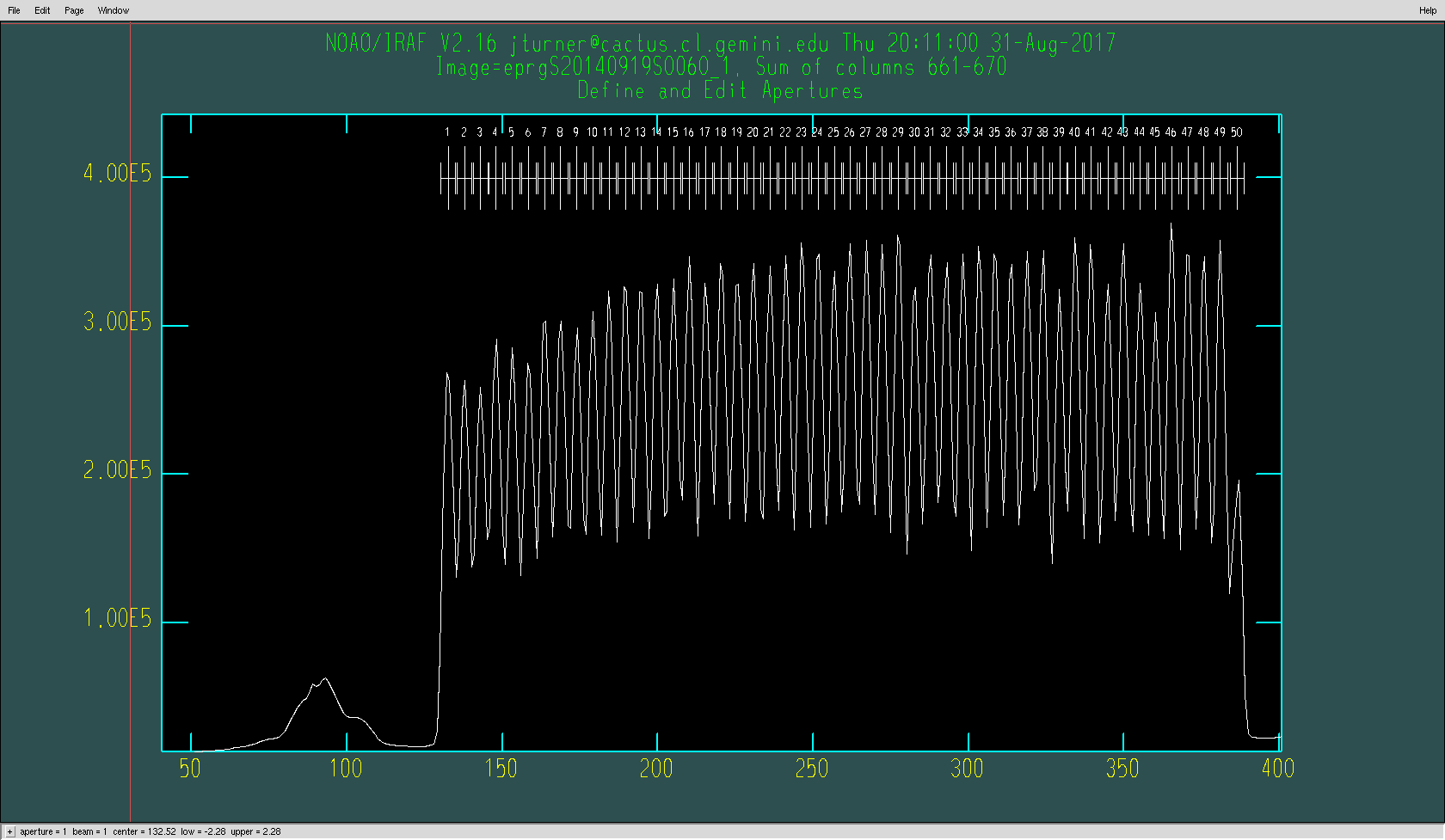
The first block of 50 fibres, after zooming interactively.
The first fibre of each block should be (N-1)*50 + 1 and the last one should be N*50 (unless those particular fibres are flagged as dead/missing in the MDF).
If the peak detection fails to find any fibre defined in the MDF – or if it does find a fibre marked as dead/missing – all subsequent identifications will be wrong. The most common reason this happens is because several fibres fall off the top of the detector and the exact number lost depends on flexure. Another reason is that some fibres with weak throughput are not always detected by apall (which I think also depends on flexure). A few broken fibres are permanently missing.
The MDF table can be modified using the TABLES task tedit:
tedit scripts$gsifu_slits_mdf_HAM.fits
Fibres are flagged as missing by setting
BEAM==-1, while good fibres haveBEAM==1. Use the arrow keys andctrl-n/ctrl-pto navigate around the table andctrl-d qto exit the task, saving your changes.There are also some gfreduce/gfextract parameters for controlling aperture identification – in particular
linecan be used to change the starting column if some artifact is misidentified as a fibre – but 90% of problems are addressed by editing the MDF to match the actual identifications. It is difficult to coerce apall to find more or fewer fibres (thethresholdparameter is rarely helpful).For the first IFU slit in this example, a permanent bright artifact at the bottom of the detector is misidentified as fibre 1. This happens because more fibres are defined in the MDF than are actually present in the image. [1] A clue is that the last aperture found is 743, which is the last good one in the MDF. Edit row 743 of the MDF file so that
BEAM==-1.You can add, delete and re-order apertures in apall if that helps you determine how to edit the MDF when unsure (press
?for help andqto return to the plot window).When finished, press
qand then keep answeringyesto the prompts. When you get another plot (showing the fibre trace), pressqagain and answerNOto skip the other traces. Answeryesto the subsequent prompts and thenqfollowed byNOwhen shown a plot of the extracted spectrum.Repeat all of the above interaction for the second IFU slit. In this case, the faint fibre 1200 at the end of the 9th block gets skipped because too few fibres are defined in the MDF. The fibre that’s actually missing from the MDF is 1493, but apall looks for the strongest peaks and 1200 happens to be weakest. Edit row 1493 of the MDF file so that
BEAM==1.If you had to edit the MDF, you will need to delete the output file(s) and repeat the above interactive extraction using the new table. First, you will need to repeat the bias subtraction & bpm steps for the flats, to attach the new MDF to the data. Once the identifications are shown correctly, you can disable
fl_interin any future runs.
The extraction step is a top candidate for replacement with a more robust Python version, but at least when it works, it works well enough.
| [1] | Your copy of the MDF has actually been altered to make the identifications fail first time in a realistic way, since this dataset happens to work with the default MDF… |